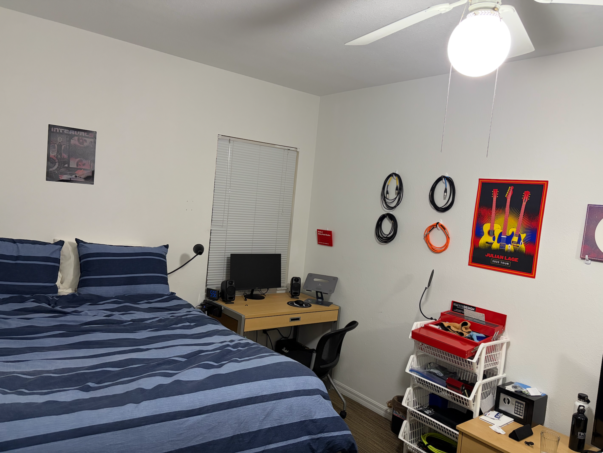
As a Music Engineering student at the Frost School of Music, I am often tasked with completing mixes and masters with short turnaround times, leaving me with no other choice than to mix in my small and untreated dorm room. Despite having a mix station setup with monitors and convertors, I always have struggled to complete mixes that translate across multiple listening environments. While one can learn to adapt to any mixing environment, my dorm at University Village is a particularly difficult space to mix due to the fact that the room is untreated.
This report presents a comprehensive acoustical analysis of “The Lake” dorm unit as a critical listening environment, so it can be used effectively for mixing purposes. The room’s geometry, RT60s, modal behavior, and early-reflections are evaluated with theoretical estimates and measured results. Theoretical estimates were derived from the geometry of the room as a “shoebox”, and are used to compare the dimensional ratios to ideal rooms, compute the axial modes, Schroeder frequency, and predicted RT60 values using the Erying-Norris equation. These predictions are then compared with data collected in Room EQ Wizard (REW) and used to develop a treatment plan and analysis of the room’s behavior.
Fig. 1: University Village “The Lake” Room Layout
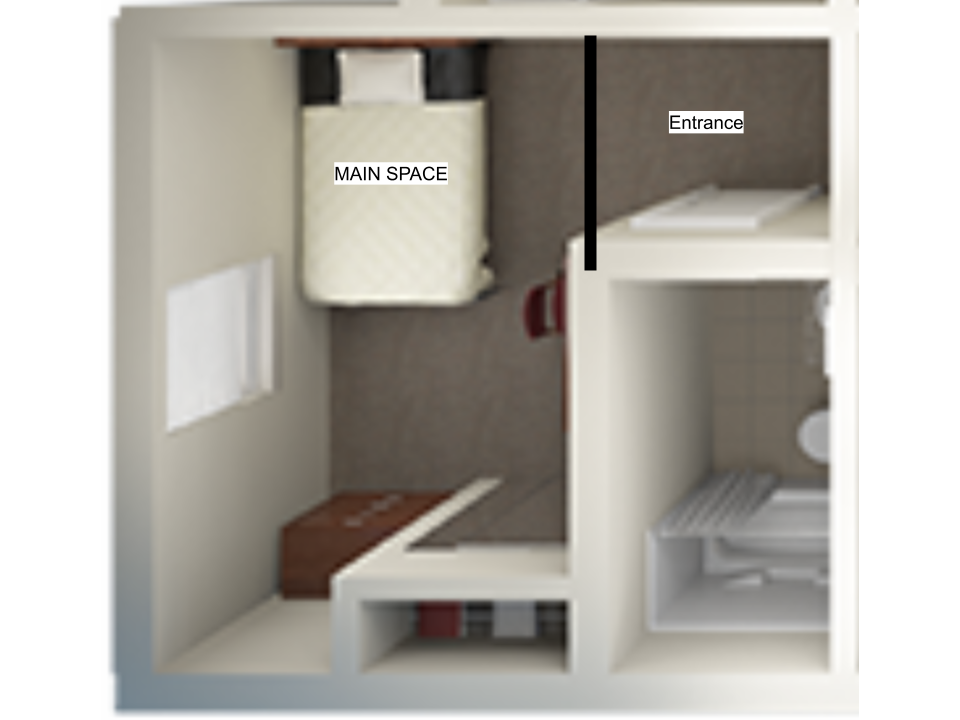
As illustrated in the floorplan displayed in Fig. 1, the room has a main space and an entrance. During the design stage of treatment, before any acoustical measurements were taken, calculations only took the main space into account.
Fig. 2: Room Dimensions in ft and m
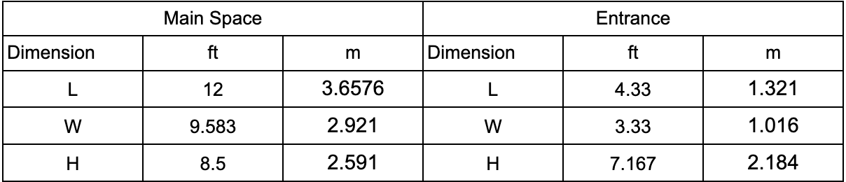
While the Entrance dimensions are to be ignored while deriving theoretical calculations for the room, it needs to be taken into account when evaluating the measured results. Due to the increased amount of space in the room, the RT60 values could be increased and there could be an increase of lower axial modes along the back wall.
Fig. 3: Room Dimension Compared to Bolt’s Area
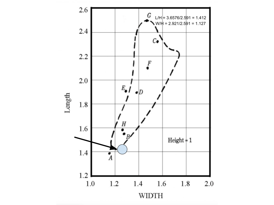
When scaling the dimensions of the main space so that H = 1, the ratio of the room narrowly falls inside Bolt’s area which means the room is almost ideal to have an even modal distribution. Despite falling on the line of Bolt’s area, the dimensions closely resemble Sepmeyer ‘A’ which is not in Bolt’s range. This means the modal response of the room may contain large nulls. When identifying possible axial modes, it is crucial to pay attention to the modal density which provides insight to the shortcomings of the room dimensions.
Fig. 4: Axial Modes Across Parallel Surfaces and Modal Spacing
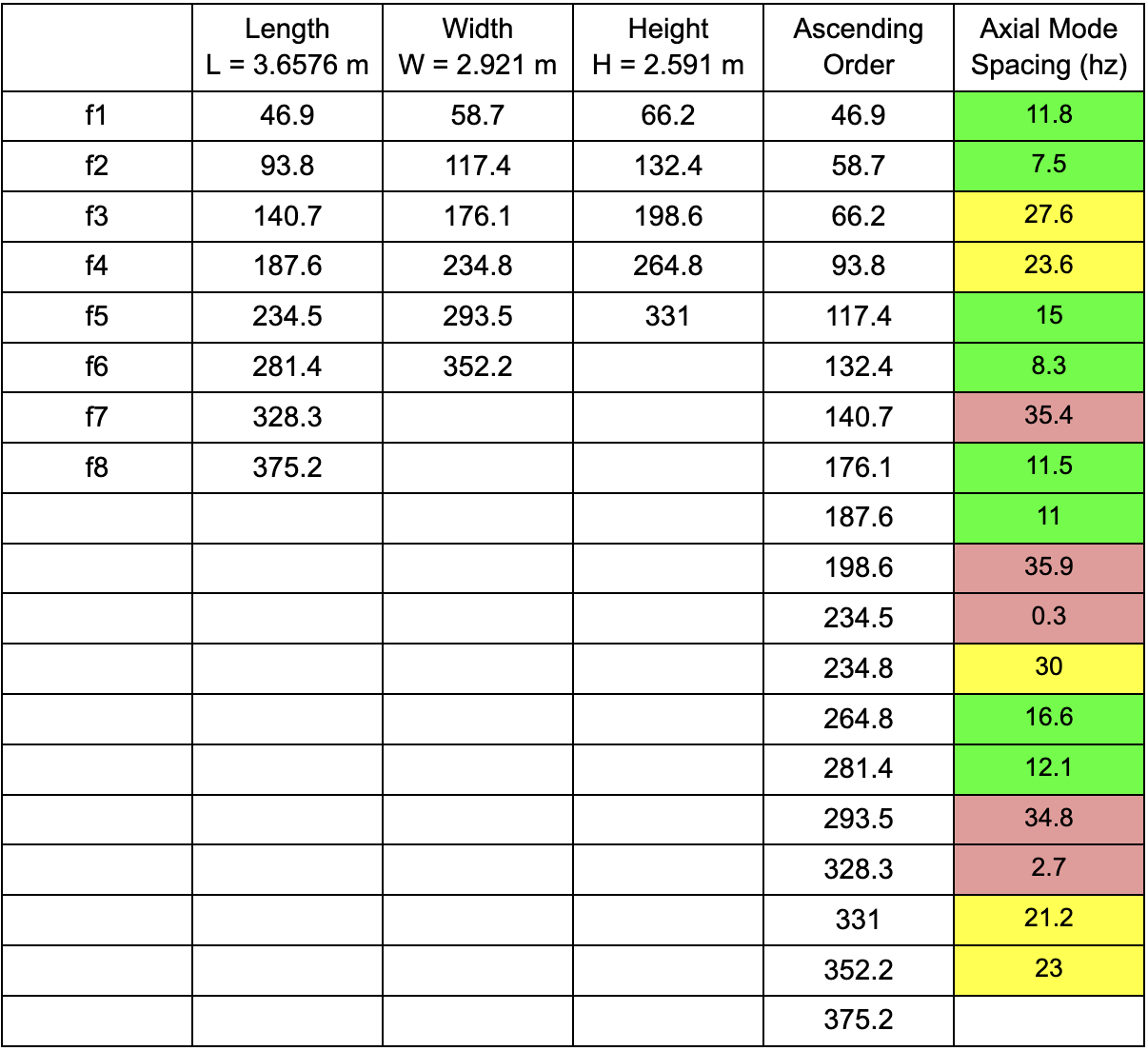
Axial modes are only evaluated up until Schroeder’s frequency at 393.4 Hz (Equation Index #1). The table in Fig. 4 lists each axial frequency between the front and back wall, side walls, and the ceiling and floor up until Schroeder’s frequency. The last two columns list out the axial modes sequentially in order of frequency and detail the spacing between each mode. The boxes highlighted in green represent ideal modal spacing that is generally around 5% of the frequency. The yellow highlighted boxes represent potential problems with spacings that are greater than 20 Hz while the red highlight indicates a significant modal spacing problem.
The densest spacing irregularities happen from 234.5 Hz-234.8 Hz and from 328.7 Hz-331 Hz. Due to these dense modes, it is expected that those frequency ranges could have reinforced resonance. This may result in an inaccurate low frequency response which accentuates those frequencies. Treating 235 Hz and 330 Hz with quarter wavelength or Helmholtz solutions is therefore recommended if the room measurements also indicate these issues.
Additionally, between 140.7 Hz-176.1 Hz, 198.6 Hz-234.5 Hz, and 293.5 hz-328.3 Hz, there are large frequency gaps between modes. These gaps can cause nulls around the frequency that is accentuated by the mode. Treating those modes individually with absorption is crucial in order to reduce the amplitude of the modes and increase the bandwidth of the absorbed mode, reducing the nulls. The low end response of the room in theory will dramatically improve by addressing the 6 frequencies with large modal spacing, and the 2 dense frequencies.
Though the modal spacing from 46.9-120 Hz is generally appropriate, there are a large number of low frequency axial modes. As a result, the reliability of low frequencies are compromised and can be accentuated or canceled based on the listening position. Since this is the frequency range that the fundamental of many bass notes exist, it can be difficult in mixing situations to monitor with a consistent bass response. One possible solution to improve the low end response would be to use corner mounted absorption since all modes terminate in corners. Additionally, panel absorbers that are strategically placed along axial modes can target specific low frequencies. If an individual frequency has a prominent peak, a Helmholtz Resonator can be used to eliminate its significant amplitude.
Fig. 5: Modal Density and Modal Spacing Plots
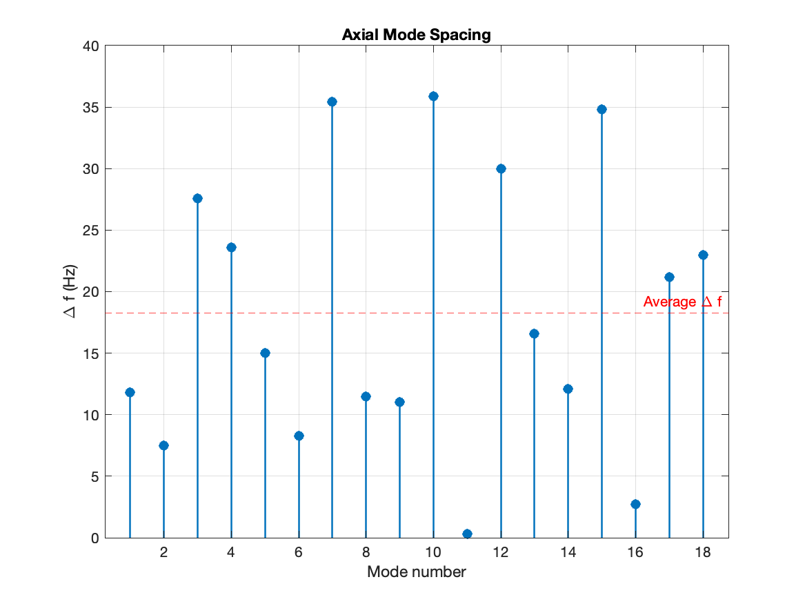
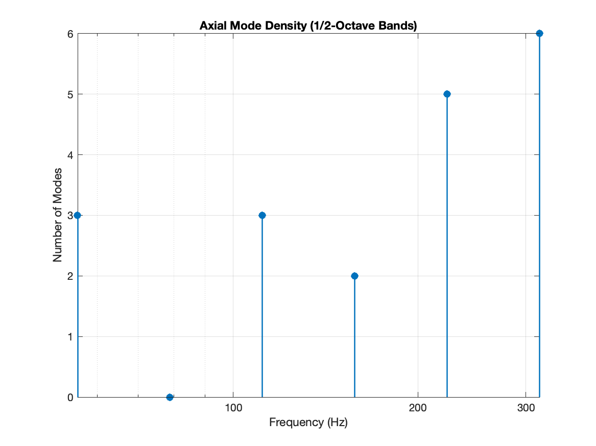
When looking at the modal density and spacing from Fig. 5, it is apparent that while the general modal density increases as frequency increases, it is not consistent between every ½ octave band. Additionally, the modal density is all over and the average spacing is not representative of the extreme outliers. This reaffirms that the frequencies with the largest and smallest modal densities need to be treated.
Fig. 6: Line Plot of Modal Density in ⅓ octave bands
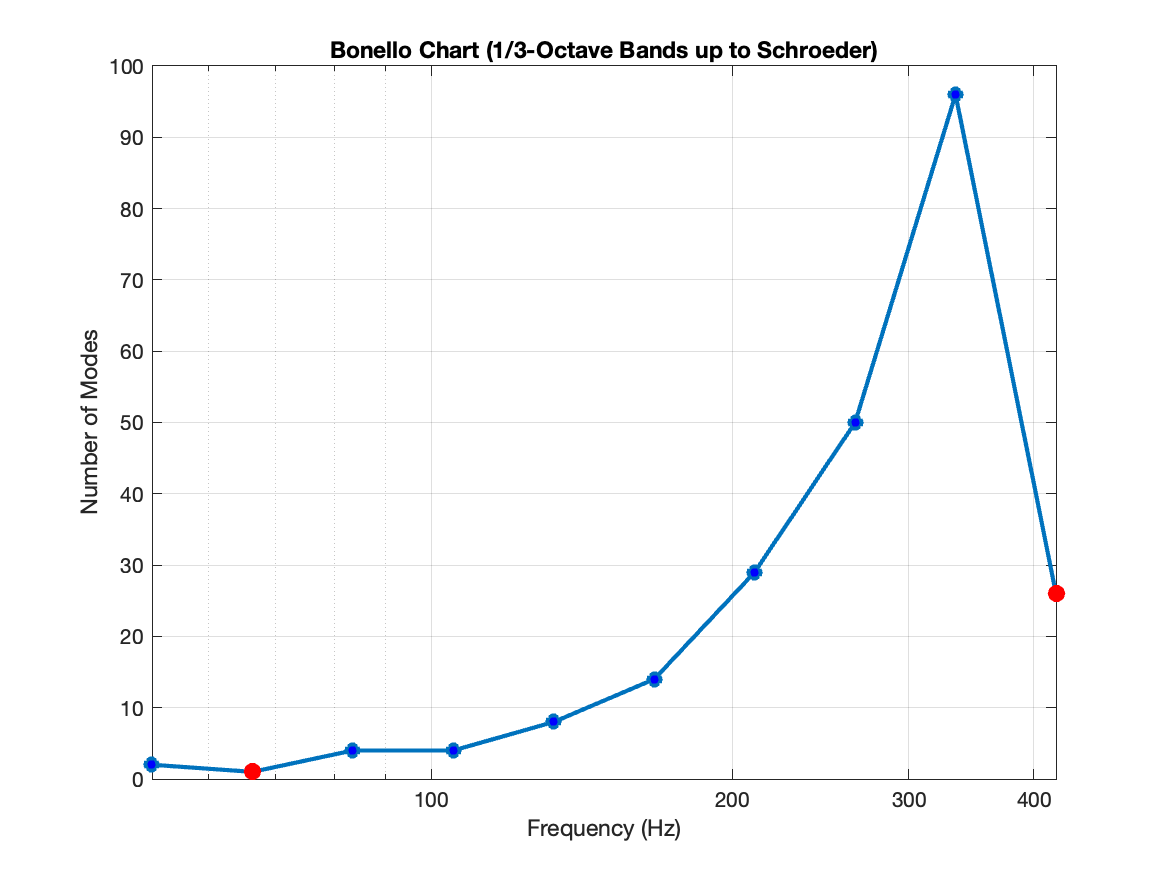
Bonello’s Criterion states that in order to prevent modal clusters and ensure even low end frequency distribution, the number of modes must stay the same or increase every ⅓ octave band. Fig. 6 was generated using more than just axial modes, it included the oblique and tangential modes up to Schroeder’s frequency. The line plot shows two red dots where the number of modes was fewer than the frequency bin before it. As a result, the dorm room fails to pass Bonello’s Criterion and when treating the room, low modes should be treated first.
When evaluating RT60s of a room, it is crucial to understand what the room is being used for, and the size of the room. Larger rooms can handle longer RTs but in this situation, the room is small and is being used as a critical listening environment. Ideally, the RT60 would be from 0.20-0.40s uniformly across all the frequency bands. It is acceptable for the low frequencies to have a slightly longer RT60 to prevent the room from sounding harsh.
Fig. 7: Absorption Coefficients and Theoretical RT60s Per Octave Band From 125 Hz - 4000 Hz
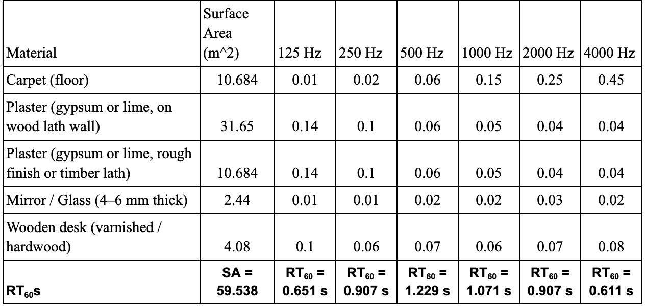
The materials listed in Fig. 7 were taken into consideration to calculate the RT60. There were bed cushions, a chair, studio equipment, and various other items in the room that are not taken into account as seen in Fig. 1. The calculated reverb times highlight a major issue from 250 Hz-1,000 Hz since it takes a long time to decay. The reverb time in the 500 Hz frequency band is almost twice as long as it is at 125 hz. In addition, the total calculated reverb time is too long for a critical listening environment to mix in. Broadly across all frequencies, there needs to be broadband absorption to lower the reverb time, with a focus on taming the low mid frequencies. One possible solution that would lead to significant improvement would be a cloud with an air gap that is at an angle to absorb a large spectrum of frequencies. 2-4” broad band panels on the side walls are also an effective choice to lower the reverb time in the room in addition to focusing on the 250-1,000Hz region. Additionally, diffusion can be used as a tool to reduce the variation in reverb times across frequencies. Drapes with many folds and an air gap over the mirror would be another decision that would lower the reverb time and would absorb a significant amount from 500-1000 Hz.
Though important, modes and reverb times do not tell the entire story of a room’s acoustics. Almost equally as important is understanding how the first reflection paths impact the frequency response where the listener is. Unfortunately, since the room is small and isn’t equipped for an ideal listening location, the mix position is in the front corner of the room as seen in Fig. 1. As a result, the speakers will have very fast first reflections off of the front wall and is likely to cause low frequency buildup in the corner.
Fig. 8: First Reflection Extra Path Length, Delay, and Relative Levels (Equation Index #4,5,6)
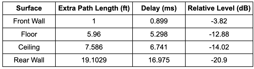
Immediately, the front wall reflection stands out as a possible problem since its delay time is under 1 ms and its relative level is only -3.82 dB when compared to the original level. Generally, once the delay exceeds 1 ms, “the notches and nulls become too dense to hear” (Bennett, slide 8). The front wall reflection is one with around 40% of the direct signal’s power and arrives under 1 ms later which is likely to cause significant comb filtering and can greatly reduce the clarity of transients. As shown in Equation index #7, the comb frequency spacing from null to null for the front wall is 1124.86 Hz. The nulls fall within critical midrange frequencies and since the reflection is at such a high volume, is likely to cause significant issues with intelligibility which is not ideal for mixing. While ideally the mixing position could be moved to help account for this, there is nowhere else to move the desk since the room’s main purpose is as a living space. Significant absorption and diffusion on the back wall is crucial to lower the first reflection level as much as possible in addition to scattering frequencies so that the direct reflection isn’t as strong.
Fig. 9: Level vs Reflection Delay Plots
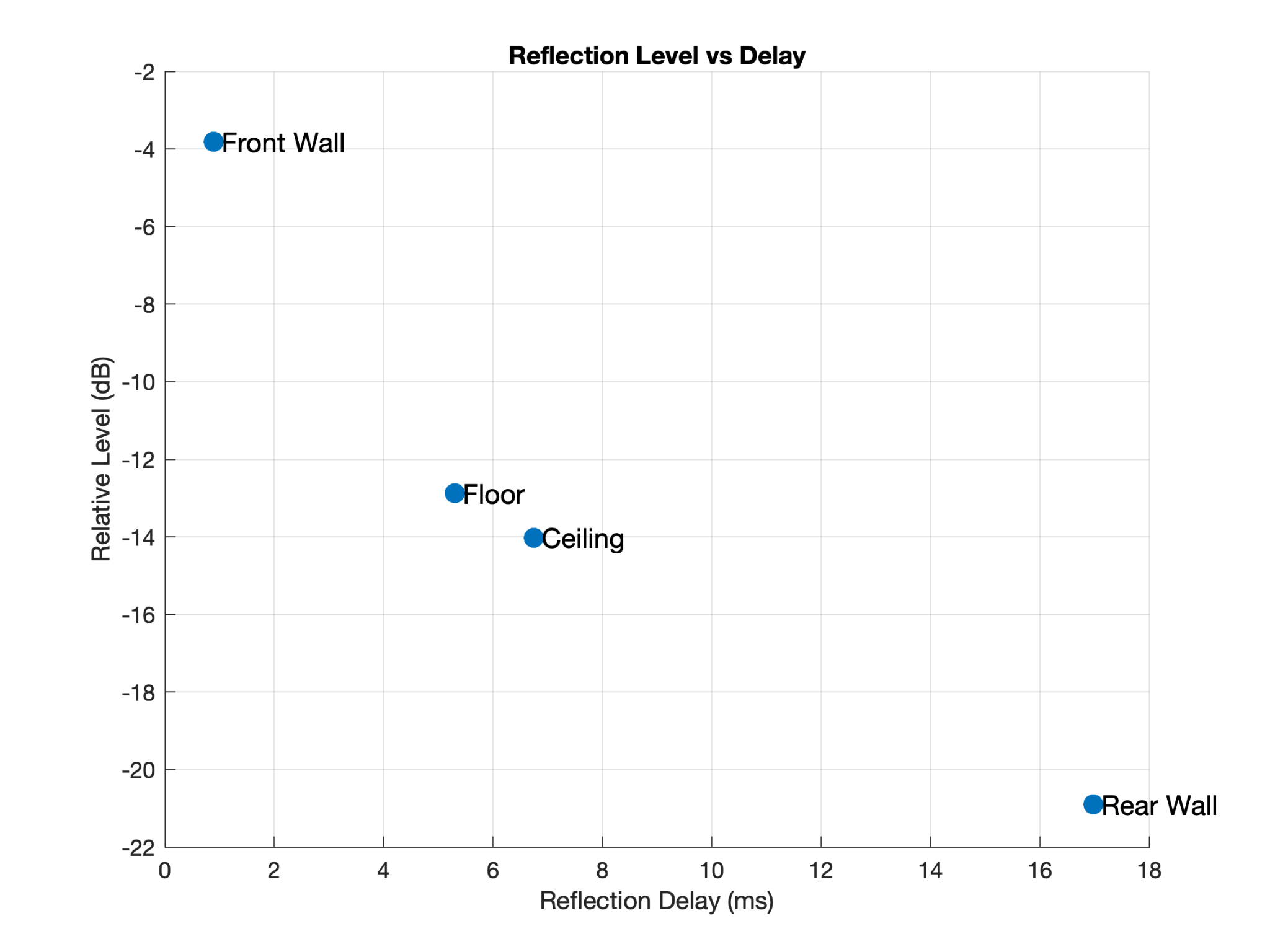
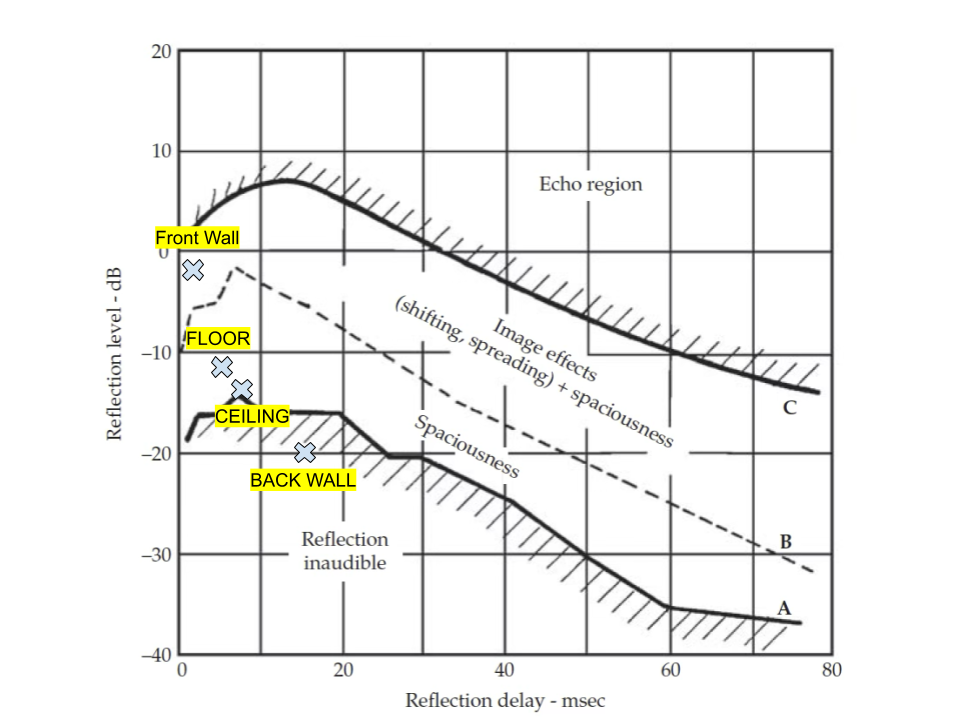
When plotting the direct reflection levels and delays, the height of the room mostly creates a spacious effect. The front wall’s image effects are unwanted as it might impact the stereo field in the mix position. The back wall is far enough away from the listening position that its direct reflection is not significant. While they weren’t measured, the side walls are likely to play a large role in the spaciousness of the room. Since the listening position is quite close to a wall, there will be an additional first reflection path with a short extra path length that should be addressed in the treatment plan.
Lastly before the measured results are evaluated, it is crucial to include that the University Village dorm has a significant amount of flutter in the room. When clapping or playing music at moderate levels, the harshness becomes noticeable quickly and is fatiguing. The short rectangular geometry of the room and reflective surfaces make the room sound like it has metallic echos which will be addressed with absorption and diffusion.
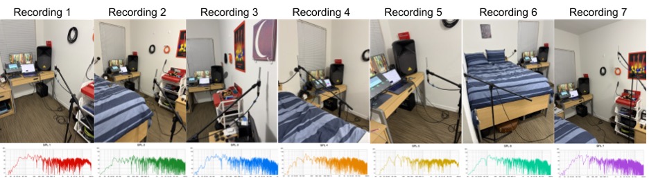
Fig. 10: Measurement Placement and Frequency Response for 7 Recordings
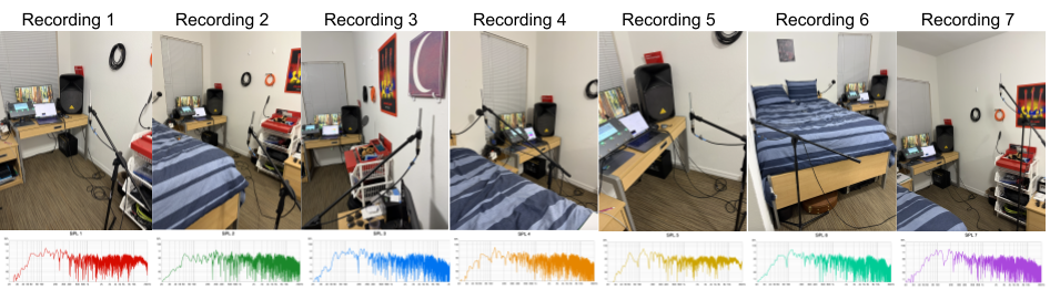
To measure the room response, a measurement microphone and soundcard was calibrated in REW. Once calibrated, the microphone was moved to 7 locations in the room that accentuated various room modes and recorded a sine sweep. Since longer sweeps have better decay resolution, a 512k length was chosen over the recommended 256k. In order to represent the frequency response as accurately as possible, the chair from the room was removed and a timer was used to have time to step out of the room before the measurement was taken. While each room location has various characteristics, many of the large problems remain consistent across each frequency response as seen in Fig. 10. Among many issues, there is often a large peak at 120 Hz, null at 140 Hz, and another significant null around 250 Hz.
Fig. 11: Average Room Response from 7 Tests
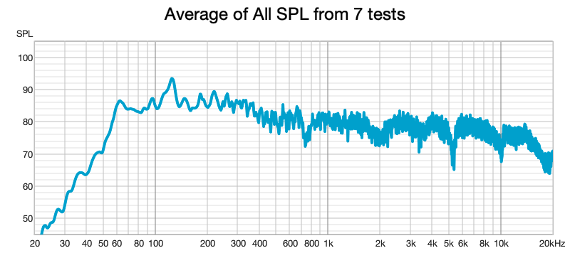
Fig. 11 displays an average from all of the measurements taken and can be analyzed as the frequency response of the room. While the rolloff in the low end likely has to do with the frequency response of the loudspeaker, there are noticeable modal issues including a null at around 40 Hz as well as boosts at 60 Hz and 95 Hz. Not surprisingly, these values are all close to axial modes listed in Fig. 4. Furthermore, the large boost at around 130 Hz that is surrounded by two nulls is also supported by the listed axial modes. At 140.7 Hz in the table, it is listed that there is a 35.4 Hz modal gap between modes which would explain the nulls that surround this clearly prominent mode. Additionally there appears to be modal resonances at 183 Hz, 218 Hz, and 262 Hz.
On top of the modal buildup below Schroeder’s frequency, there is apparent comb filtering with visible nulls at 740 Hz, 1.3 kHz, 2 kHz, 4 kHz, 5.3 kHz, and 10 kHz. As previously discussed, these are likely due to the reflections from the front wall and other first reflections. When treating the room, it will be essential to try to increase the delay time and decrease the amplitude of reflections from the front wall.
Fig. 12: T30 Reverb Time in Octave Bands and Chart Converting to RT60 Values
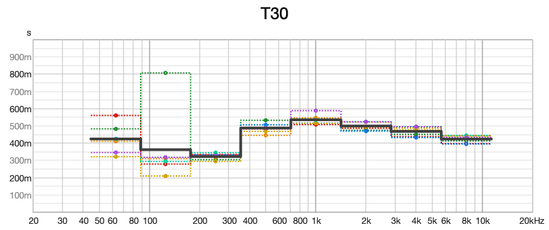
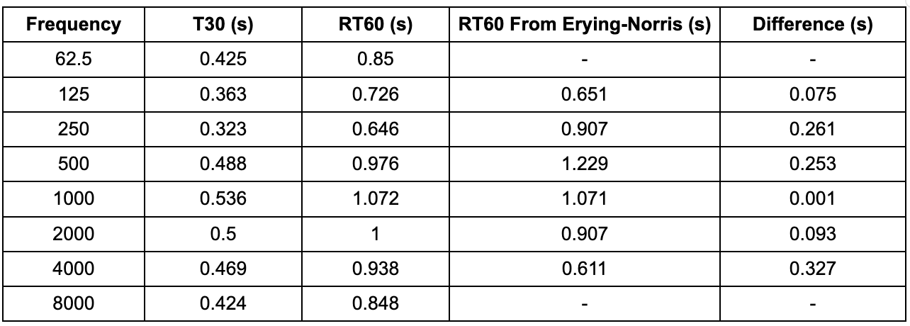
As displayed in Fig. 12, the calculated reverb behavior is impressively similar to the calculated RT60 values from the Eyring-Noris equation. In fact, at 1,000 Hz, the measured value was only 0.001 s higher than the calculated value. The largest discrepancy is from the predicted reverb times from 250-500 Hz and at 4000 hz. However, it works in the favor of the treatment plan since the 250-500 Hz frequency range was measured as a faster RT60 than it was originally calculated. While the overall reverb time of the room needs to be lowered across all frequencies, there must be careful treatment to significantly lower the reverb time from 500-2k Hz. As previously mentioned, it is acceptable for the low frequencies to have a slightly higher reverberation than the higher frequencies. Equation Index #8 proves that the bass rise in this untreated room is 0.6699 which is short of the recommended range of 1.1-1.45. This further indicates the importance of reducing the mid frequencies in the room to prevent it from sounding harsh.
Fig. 13: Energy-Time Curve Detailing How Sound Arrives Over Time
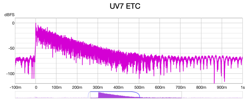
As previously referenced, there is an audible high frequency flutter that is immediately noticeable when monitoring music and is audibly fatiguing in the University Village dorm. When evaluating the energy-time Curve in Fig. 13, it is apparent that there is a quick repeating oscillation that appears to be evenly spaced from 100 ms to 1,000 ms. Its even character and repetition through the entire decay is indicative of this audible flutter. Fig. 13 was derived from recording 7, which, as shown in Fig. 10, was in the center of the room. Of all recordings, this is the most likely to show the behavior of the flutter echo in the room since it is equidistant to all parallel surfaces.
Fig. 14: Additional Sabins of Absorption to Meet Target RT60 Values (Equation Index #9)
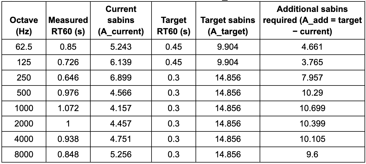
In summary, treatment will be necessary to reduce excessive mid-frequency reverb time, control strong first reflections off of the front and side wall, eliminate harsh flutter echo, and mitigate low frequency modes in order to create a balanced and accurate listening environment. Specifically, 250 Hz-1,000 Hz needs to have a significant reduction in reverberation, the axial modes from 46.9 Hz-120 Hz need to be reduced, the boosts from dense modes around 240 Hz and 330 Hz need to absorbed, and the nulls from 140–176 Hz, 198–234 Hz, and 293–328 Hz need to reinforced. Diffusion needs to be implemented to address the flutter between parallel surfaces and broadband absorption will be used to reduce the prominent first reflections. As detailed in Fig. 14, the additional sabins required to reach a target RT60 of 0.3 s averages around 10.39 sabins for frequencies from 500-4,000 Hz.
In order to create a uniform bass response and reduce gain buildup in sub frequencies from 30-90 Hz, 27” corner bass traps will be installed from in both corners on the front wall, and the corner nearest the listening position on the back wall. While these are massive traps, they only take up 19” on each side wall and take up around 3.3% of the floor space. At 27 inches, these will do a fantastic job absorbing 125 Hz and due to the absorber’s triangle shape, it will absorb a broad band of frequencies at quarter wavelength. It is difficult to directly address lower frequencies such as 50 hz because it would take 67.5 inches of porous absorption. However, since all modes terminate in corners, the corner mount will do an excellent job at reducing low frequency buildup in the room. Additionally, a 10” airtight membrane absorber with internal lining, ¾” medium density fiber, and added mass will be installed on the back wall to absorb the mode at 46.9 Hz and reduce room modes at 58.7 Hz.
It is essential to have broadband low frequency absorption on the front wall in order to account for its close proximity to the speakers. If the desk is backed off of the wall, a 4 inch absorber with a 4 inch air gap can line the front wall absorbing as low as 170 Hz. Since low frequencies aren’t directional the same way high frequencies are, there is more low end that will be directed towards the front wall than high frequency content which directionally travels towards the listening position.
Panels will be placed to reduce the overall reverb time in the room, especially focusing on 500-4,000 Hz. Using the absorption coefficients of Rockwool, fifteen 2’x4’x4” panels with a 4” air gap will be placed in order to achieve the optimal absorption count. 4 panels will be placed with even spacing on the front wall. 3 panels will be placed on each side wall, at the height of the tweeter. It is essential that one of the panels covers the location of the reflection point on each side wall. This can be located if one person sits in the listening location and the other walks with a mirror until the listener can see the tweeter reflected on the mirror. On the back wall, 3 panels will be placed in the center of the wall with small gaps in between. The sharp edges of the panels also diffract the sound into adjacent absorbers to help reduce the reverb time. The final 2 panels are to be reserved and placed accordingly after measuring the room again. They can be used placed over severe reflections or at locations of modal buildup.
A cloud is to be placed over the listening position at an angle so that it can absorb a broad band of low frequencies and lower the first reflection from the ceiling. A 4’x6’ cloud is enough to improve the low end response without being too large that it is in the way of the ceiling fan. Lastly, drapes with many folds will be installed with a dorm friendly tension rod over the back mirror to exceed the expected absorption since panels are not always ideal. With absorption coefficients up to 0.75 at the 1,000 Hz band, the drapes will improve the mid frequency RT60 compared to the 0.02 absorption coefficient of a mirror. The drapes can be opened and closed which makes the room more flexible.
In order to address the dense modal clusters at 235 Hz and 330 Hz, membrane absorbers will be used. A sealed box with a flexible membrane tuned to 235 hz will be placed on the back and side wall and similarly, one tuned to 330 Hz will be placed on the other side wall and ceiling. These will reduce the amplitude of the large peaks and broaden the resonances so it can be absorbed by the panels. This is more convenient in a dorm room than creating a Helmholtz resonator.
In order to address the flutter echo in the room, a skyline diffuser with rectangular shapes will be placed along the back wall above the panels. This will help scatter mid and high frequencies for an even and smooth reverb time. The panels along the walls also disperse sound with their sharp edges. As a result of absorption panels, tuned membrane panels, corner bass traps, the cloud, drapes over the mirror, and back wall diffusion, the University Village dorm is expected to have more accurate and consistent results when used as a mixing environment.
Fig. 15: Room Impulse Response Simulation In Matlab Using “ray-tracing” Algorithm
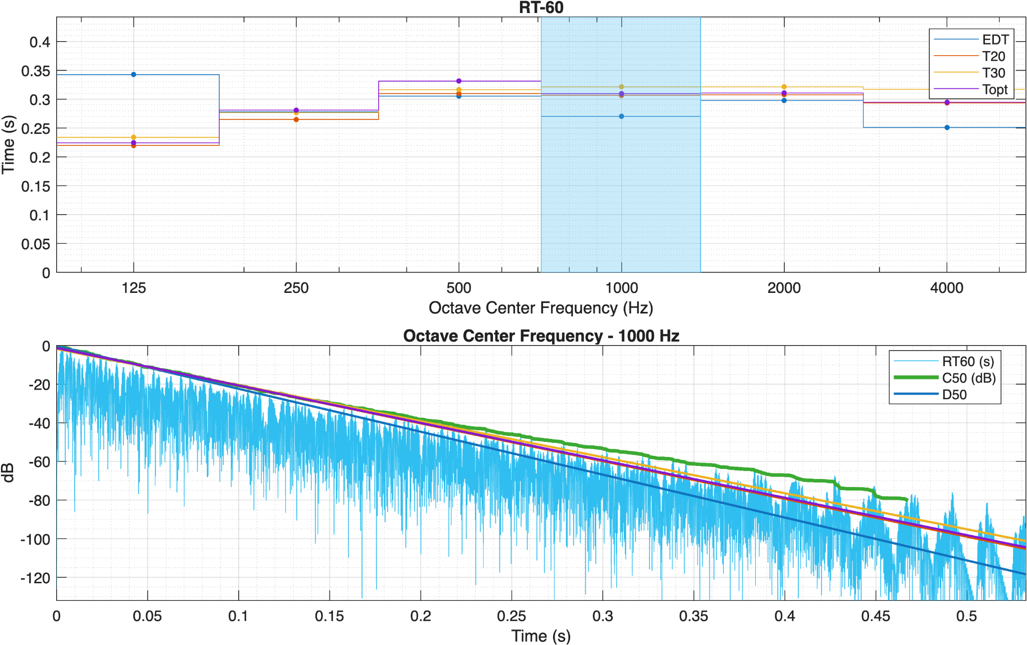
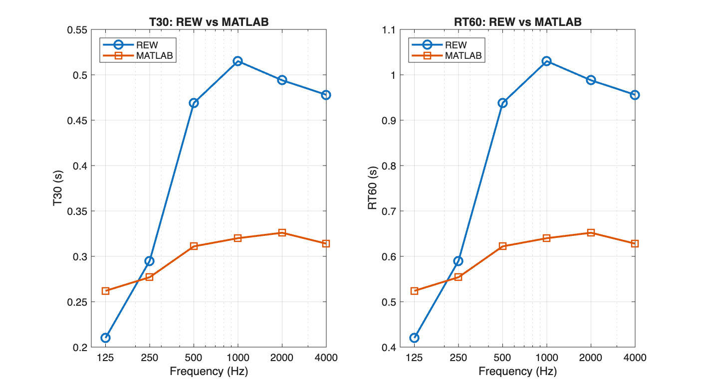
Fig. 15 displays the RT60 analysis of a generated room impulse response using Matlab. When comparing to the measured RT60 values found using REW, it is clear that the reverb times of the impulse are substantially lower. However, the behavior across frequency bands remains fairly consistent aside from the significant peak at 1 kHz. This could be due to the fact that the impulse response simulation doesn’t take into account any of the objects in the room that scatter sound. In addition, the entrance of the room is not taken into account in the Matlab simulation.
Fig. 16: Overlay Plot of C50 and D50 clarity
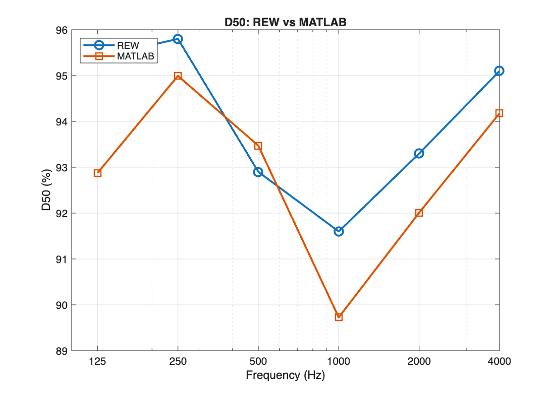
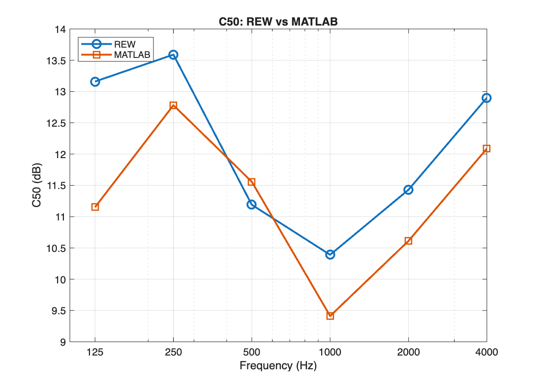
Contrasting from the RT60 measurements, the clarity measurements from Matlab’s room impulse response simulation is similar to the measured clarity in the room. The C50 is an “early to late ratio in dB” (REW) that indicates speech clarity. This room has high C50 values meaning the dB SPL in the first 50 ms is significantly louder than after the first 50 ms. The D50 reinforces this ratio as a percentage of energy. This means that a high percentage of the energy dissipates in the first 50 ms. The dip at 1 kHz explains why there is a longer RT60 in that frequency range.
Equation Index
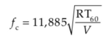
#1 Schroeder’s Frequency
RT60(1000 Hz) = 0.651, V = 27.6719
Fc(1000)= = 393.4 hz
#2 Axial Mode Sample Calculation
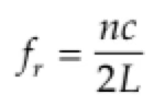
C = 343 m/s, L = 3.5576 m
fr = = 46.9 Hz
#3 Sample RT60 Calculation Using Erying-Norris Equation
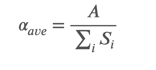
= 0.1086
V = 27.6819 m3, S = 59.538 m2
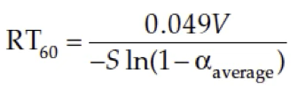
RT60(125 Hz) = = 0.651 s
#4. Sample Calculation for Floor Reflection Extra Path Length
Extra Path Length = Distance of Reflection - Direct Path
Speaker (center) = (x, y, z) = (0.50 ft, 7.70833 ft, 3.83333 ft)
Listener = (x, y, z) = (2.44856 ft, 7.70833 ft, 3.83333 ft)
Direct distance =
= 1.948 ft
Distance of Reflection = 2 *
Floor Reflection = (x, y, z) = (1.47428 ft, 7.70833 ft, 0.0 ft) - Halfway between listener and floor
= 7.909 ft
Extra Path Length = 7.9096 - 1.948 = 5.96
#5. Sample Calculation for Floor Reflection Delay
Delay = = 0.005298 s = 5.298 ms
#6. Sample Calculation for Floor Reflection Relative Level
Relative Level =
Relative Level = = -12.88 dB
#7. Front Wall Reflection Comb Filtering
Comb Frequency Spacing = Fnull2 - Fnull1
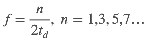
Fnull1 =
Fnull2 =
1687.289 - 562.429 = 1124.86 Hz
#8. Bass Rise from Calculated RT60
BR =
BR = = 0.6699
#8. Sample Calculation for Target Sabins of Absorption
A =
A(62.5 Hz) = = 5.243 sabins
A(Target) = = 9.904 sabins
Additional Sabins Required = 9.904 - 5.243 = 4.661 sabins
Sources
Matlab Help Center. "Room Impulse Response Simulation with Stochastic Ray Tracing." Mathworks.com, www.mathworks.com/help/audio/ug/room-impulse-response-simulation-with-stochastic-ray-tracing.html. Accessed 5 Dec. 2025.
Matlab Help Center. "Room Impulse Response Simulation with Stochastic Ray Tracing." Mathworks.com, Mathworks, www.mathworks.com/help/audio/ug/room-impulse-response-simulation-with-image-source-method-and-hrtf-interpolation.html. Accessed 5 Dec. 2025.
JCW Acoustic Supplies. "Sound Absorption Coefficient Chart (125 Hz–4 KHz)." Acoustic Supplies, 6 Oct. 2025, www.acoustic-supplies.com/absorption-coefficient-chart/. Accessed 5 Dec. 2025.
"web_absorption_data_eng." https://www.acoustic.ua/st/web_absorption_data_eng.pdf, acoustic.ua, Accessed 5 Dec. 2025.
REW. "Clarity Graph." REW - Room EQ Wizard Room Acoustics Software, www.roomeqwizard.com/help/help_en-GB/html/graph_clarity.html. Accessed 5 Dec. 2025.
Music City Acoustics. YouTube, 10 Mar. 2022, www.youtube.com/watch?v=HYMQ6M-Z5rM. Accessed 5 Dec. 2025.