
The Ear Acoustics Simulator is an interactive web application for exploring simplified models of hearing. It extends an outer-ear model with a middle-ear simulation and a binaural renderer, with visualized responses and real-time audio playback.
Middle Ear Simulation Extension Documentation
Objective and model scope
The middle-ear model extends the outer-ear simulator through a signal path from the pinna and concha, through the ear canal, eardrum, and ossicles, to a cochlear load. The application displays and plays the outer-ear response, middle-ear response, and their combined response in real time. The model combines stages by multiplying transfer functions, without modeling loading between stages:
H_total(f) = H_outer(f) × H_middle(f)
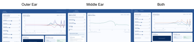
Figure 1. Outer, middle, and combined magnitude responses in the web application.
Middle-ear circuit and verification
The circuit is implemented as impedance subsystems for the cavity, eardrum, ossicles, joint, and cochlea. The output transfer function is the pressure ratio from input to cochlear load:
Z_cavity = (Z_Cp + Z_La + Z_Ra) || Z_Rm || Z_Ct
Z_eardrum = Z_CD1 + (Z_LD || (Z_CD2 + Z_RD2)) + Z_RD1
Z_ossicles = Z_CO + Z_LO + Z_RO
Z_load = Z_joint || Z_cochlea
Z_middle = Z_cavity + [Z_eardrum || (Z_ossicles + Z_load)]
H_middle = (Z_after_A / Z_middle) × (Z_load / (Z_ossicles + Z_load))
Code checks at 1 kHz compared the real and imaginary components of each subsystem and verified the branches in the impedance equations. The checks also confirmed that resistor impedance stays constant as frequency changes, while inductor impedance rises and capacitor impedance falls with frequency. The current through a capacitor is 90 degrees out of phase with voltage. The report records 21 automated checks before the production build.
Circuit and component values
The implementation follows the provided Zwislocki-style middle-ear circuit. Baseline cavity impedance and compliance values were derived from the response in Figure 3 of Zwislocki’s 1962 paper, with the simplified malleus and ossicle behavior based on its discussion on page 1517. Cochlear inertance was set to zero as a model simplification.
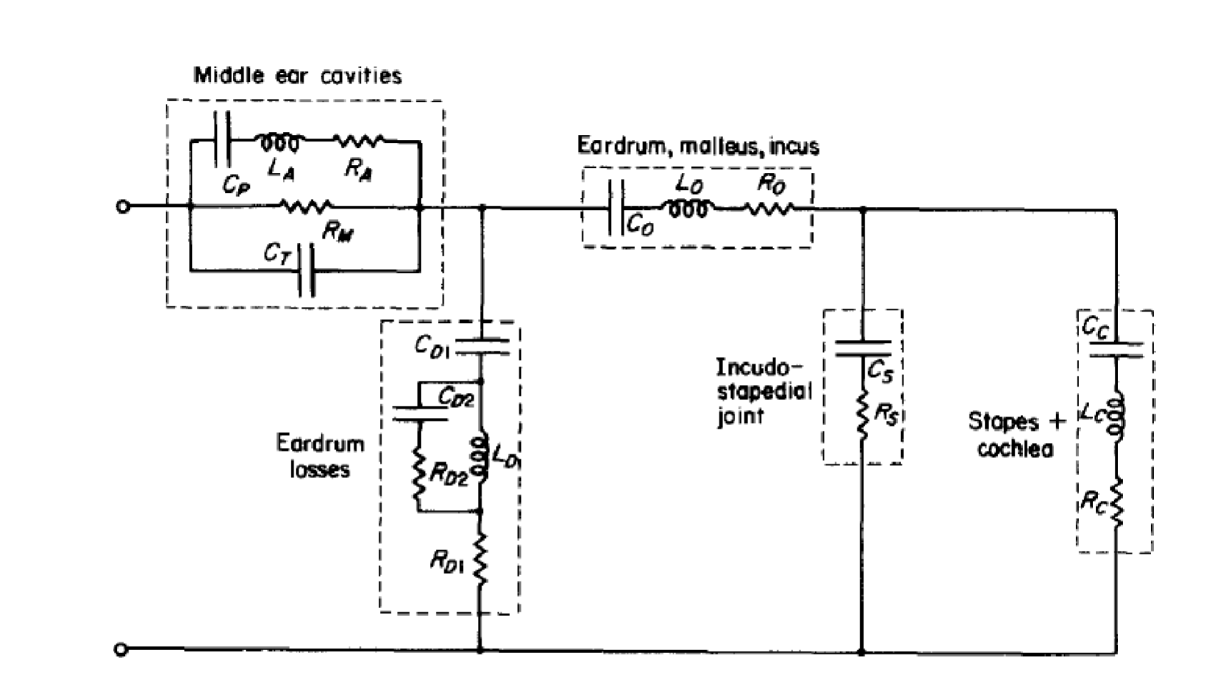
Figure 2. Zwislocki-style middle-ear circuit diagram.
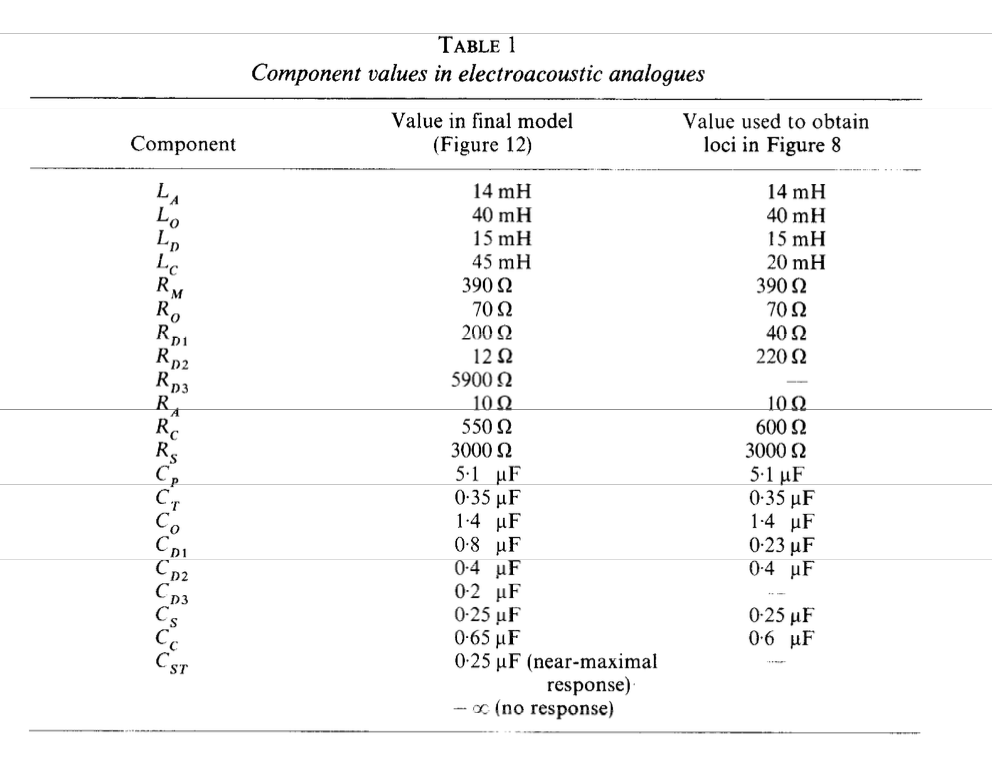
Component values used in the middle-ear model.
Source: Zwislocki, “Analysis of the Middle Ear Function. Part 1: Input Impedance” (1962).
Controlled parameter experiments
Each experiment changes one middle-ear parameter while resetting the remaining controls to the OME scenario.
Ossicular inertance
Ossicular inertance was changed from 40 to 60 mH, a 50% increase. The prediction was that the higher inertance would attenuate high frequencies beyond the middle-frequency peak. The peak moved from 871 Hz to 752 Hz. Relative to baseline, the response changed by −1.32 dB at 2 kHz and −2.00 dB at 4 kHz. The high-frequency roll-off moved as expected, alongside a slight increase around the broad response peak.
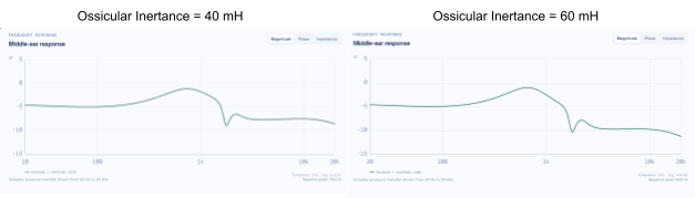
Figure 3. Response comparison for 40 mH and 60 mH ossicular inertance.
Eardrum compliance
The eardrum compliance parameter CD1 was changed from 0.8 to 0.10 μF. The prediction was that changing capacitance would attenuate the broad peak. The peak moved from 745 Hz to 726 Hz, and its magnitude changed from −1.11 dB to −1.16 dB. At 1 kHz, the response was −0.21 dB relative to baseline.
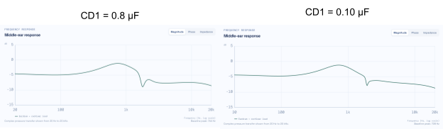
Figure 4. Response comparison for the two CD1 settings.
Ossicular loss
Resistance R0 was changed from 70 to 300 Ω. The prediction was that increased resistance would dissipate more energy and reduce the broad peak. The peak moved from 745 Hz to 649 Hz, and its magnitude changed from −1.11 dB to −4.11 dB. At 1 kHz, the response was −2.69 dB relative to baseline. The larger resistance reduced the broad peak as expected.
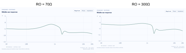
Figure 5. Response comparison for 70 Ω and 300 Ω ossicular loss.
OME transfer scenario
The application includes a small-child otitis media with effusion (OME) sensitivity scenario. As severity increases, the model reduces eardrum and joint compliance while increasing ossicular inertance and loss. Above zero severity, it overlays baseline and OME responses and applies the same profile to playback.
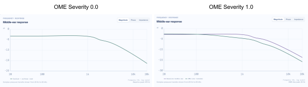
Figure 6. Baseline response and OME response at two severity settings.
Engineering notes and limitations
The circuit interpretation began with the verified topology in the supplied notes rather than using AI to infer alternate circuits from the published response. The component values were later supplied and implemented, confirming a similar baseline without arbitrary values. During app development, an initial custom FFT filtering approach caused playback glitches; replacing it with fft.js produced accurate frequency response and playback.
This is a first-order approximation, not a complete anatomical model. The stages do not include loading between them, and multiplying the transfer functions does not represent the ear’s full anatomy or impedance changes. The OME scenario is not clinically calibrated and is not for diagnosis.
HRIR Generator
Purpose and model
The binaural renderer uses a source direction and baseline ear geometry to produce left and right head-related transfer functions (HRTFs), converts them into head-related impulse responses (HRIRs), then convolves the HRIRs with a mono source to create stereo audio.
Each ear’s response combines the direction-dependent outer-ear response, a small elevation-dependent reflection, frequency-dependent head shadow, and phase delay. Interaural timing is estimated from the geometry:
ITD = head diameter / speed of sound × sin(azimuth)
A shared 1 ms delay keeps both HRIRs causal without changing interaural timing. HRTFs are converted to left and right HRIRs by an inverse FFT at 48 kHz. Applying the middle-ear transfer function to both channels changes their spectrum without creating an interaural time difference. Cross-correlation estimates the HRIR interaural time difference; positive values indicate a source to the left and negative values a source to the right.
Procedure and comparison cases
For each comparison, the fixed case was loaded in the Binaural HRTF view, the predicted and HRIR-estimated timing were recorded, and the HRTF, HRIR, and interaural-level-difference plots were exported. Baseline geometry was restored before each case.
- Median plane: 0° azimuth, 0° elevation; predicted ITD 0.000 ms and estimated ITD 0.000 ms. Left and right HRTFs match, so horizontal localization is not driven by interaural timing.
- Lateral left: 75° azimuth, 0° elevation; predicted ITD 0.493 ms and estimated ITD 0.500 ms. The right ear becomes more attenuated at higher frequencies, producing a high-frequency head shadow.
- Elevated front: 0° azimuth, 45° elevation; predicted and estimated ITD 0.000 ms. Elevation changes delayed reflections while preserving the plane timing, demonstrating a spectral cue.
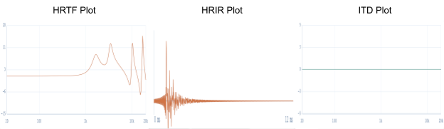
Figure 1. Median-plane HRTF, HRIR, and ITD results.
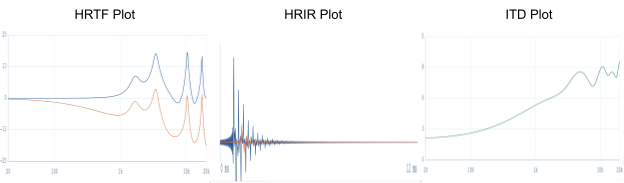
Figure 2. Lateral-case HRTF, HRIR, and ITD results.
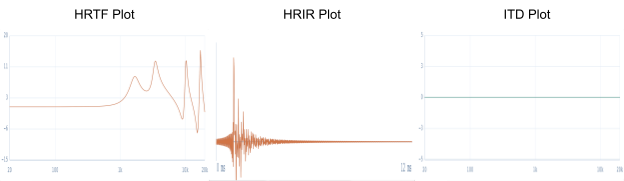
Figure 3. Elevated-front case result.
The report validates the expected behaviors: interaural time difference grows with azimuth, level differences grow at higher frequencies, and elevation changes spectral peaks and notches. The model is simpler than a measured, listener-specific HRTF and does not reproduce individual ear structure, room reflections, or head motion.
Binaural audio example and engineering notes
A short pink-noise source was rendered through the left and right HRIRs using linear convolution. The report links to the HRIR file and rendered audio.
AI assisted with model organization, testing, and interface implementation. During validation, an initial case loader merged a physical SourceDirection object directly into UI state. The UI expected azimuth and elevation values, while SourceDirection used azimuth degrees and elevation degrees; the mismatch caused the case buttons to remain at zero degrees. The state mapping was corrected during development.