
Matlab:https://drive.google.com/drive/folders/1Py__ChNX8KZobDo_qVh9si36xCWuhEmX?usp=sharing

The Lundy Liquid Pre FX plugin is a ‘wah’ and drive effect that is designed to be placed before an amplifier plugin for guitar signals. The tanh distortion algorithm models drive pedals such as the Ibanez Tube Screamer and is a powerful device to boost the input and gain of a guitar signal going into an amplifier. The Wah pedal is modeled based on the schematic of the Dunlop CryBaby GCB-95 pedal and uses exact component values and transfer functions as the schematic. The drive section features switchable antiderivative antialiasing to attenuate harmonics that can alias. Additionally there is a Chebyshev polynomial black box model of the tanh distortion that can be enabled and disabled.
Fig 1: Spectrum: Harmonic Magnitude With and Without ADAA Using a Test Signal of 10 kHz
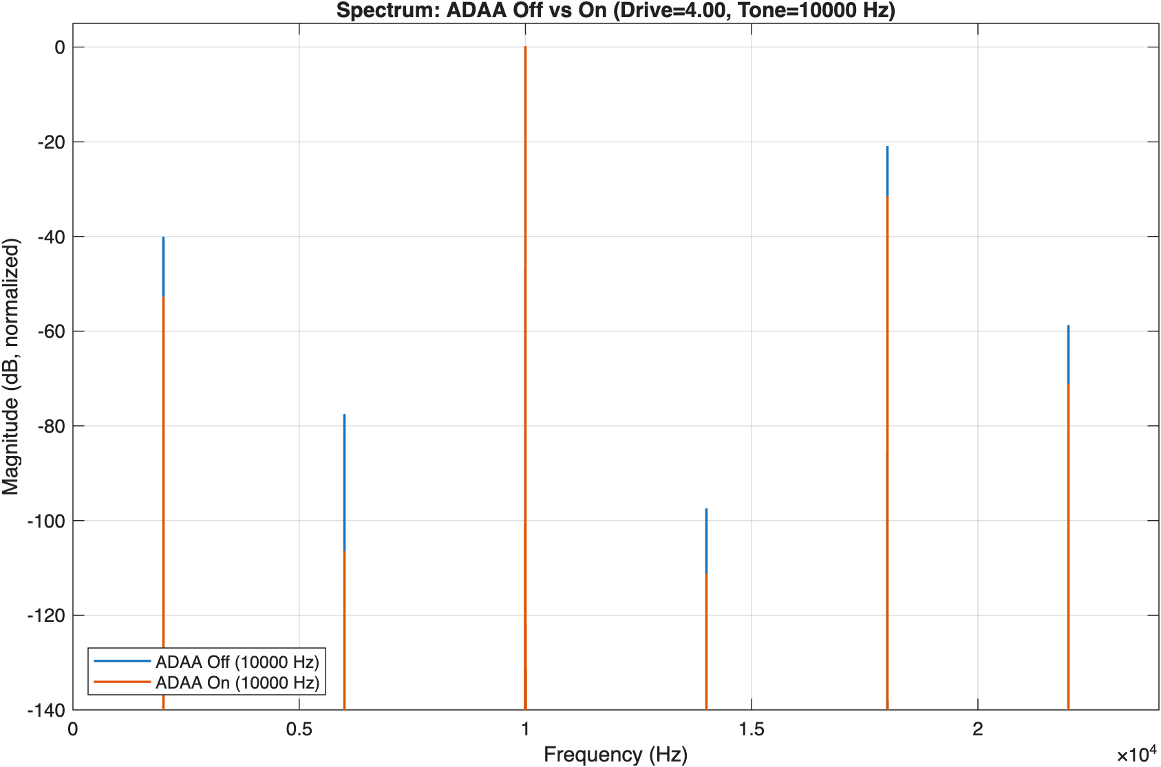
Fig 2: ESS Input and Output Through Tanh Nonlinearity and ADAA
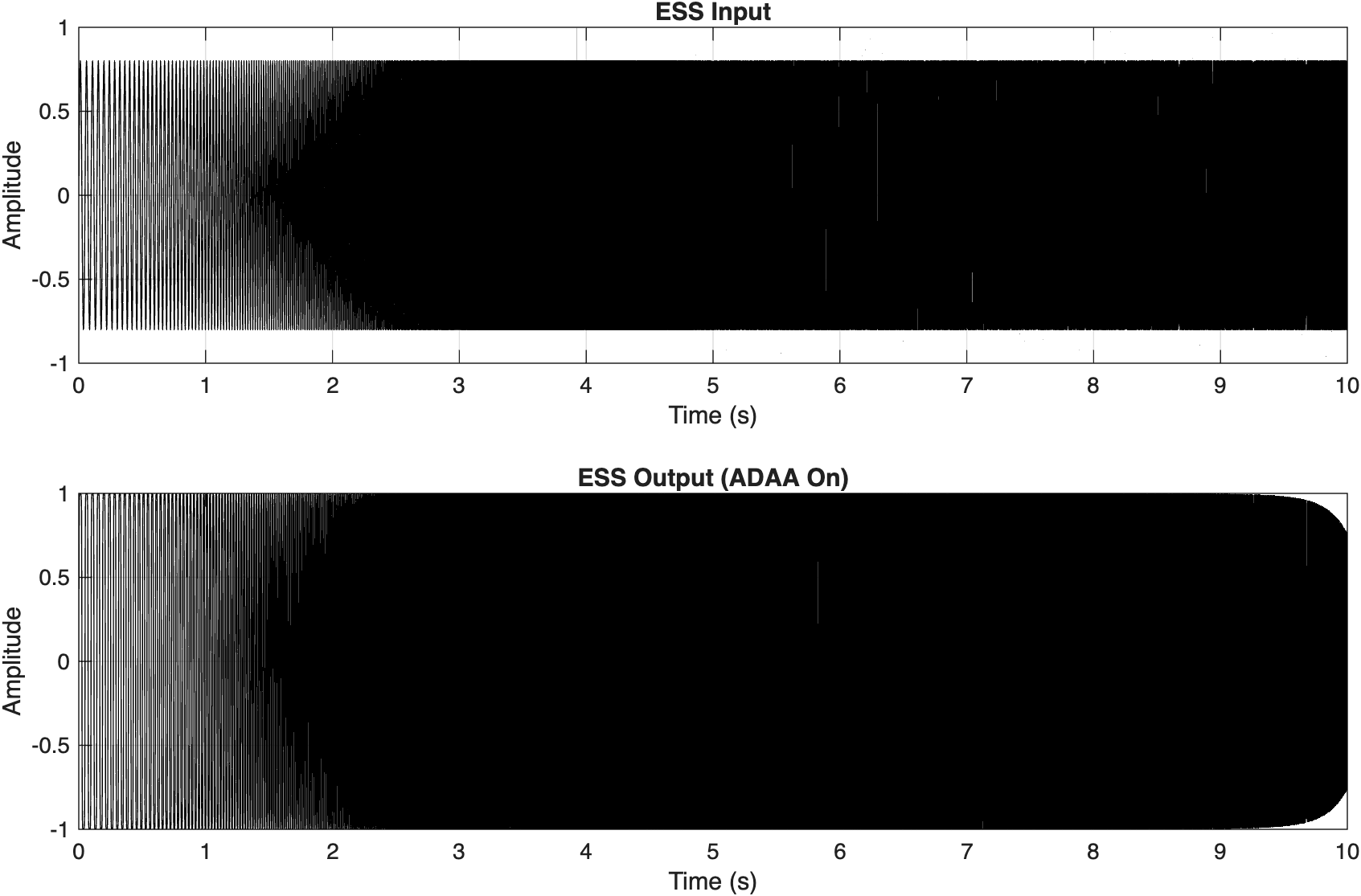
The ESS was sent through the tanh clipper with the ADAA algorithm. The wah section of the plugin was off during the following measurements. As a result, there is a significant boost in amplitude and the signal rolls off at the end of the sweep due to the ADAA.
Fig 3: Impulse Response After Deconvolving ESS (Linear Impulse Response)
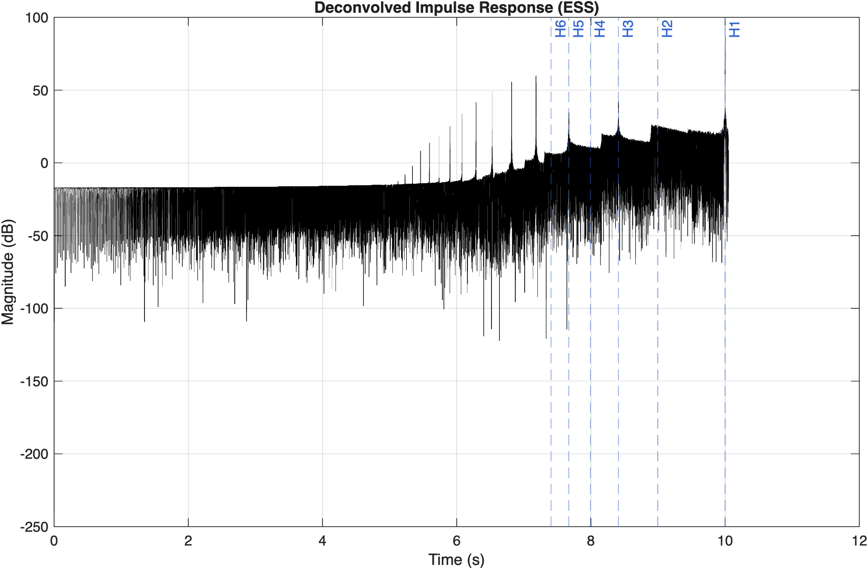
The deconvolved impulse responses show the spacing and magnitude of each harmonic that was passed through the tanh clipper. Since the harmonic separation remains clean throughout the deconvolved impulse response, it is simple to extract them as seen in Fig. 4 and apply it to the Chebyshev Hammerstein model.
Fig 4: 6 Harmonic Impulse Responses
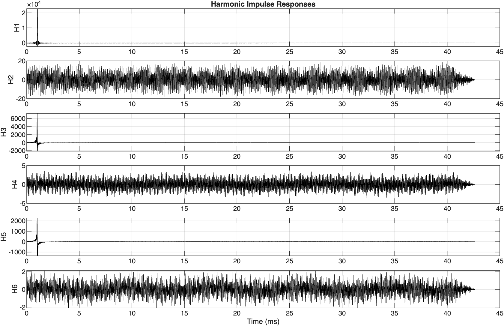
Notice how the odd harmonics show a clear impulse response while the even harmonics appear as noise that oscillates between +- 2. This is additional representation that the impulse responses in this Chebyshev model are representing the odd harmonics in the system.
Fig 5: Harmonic Levels
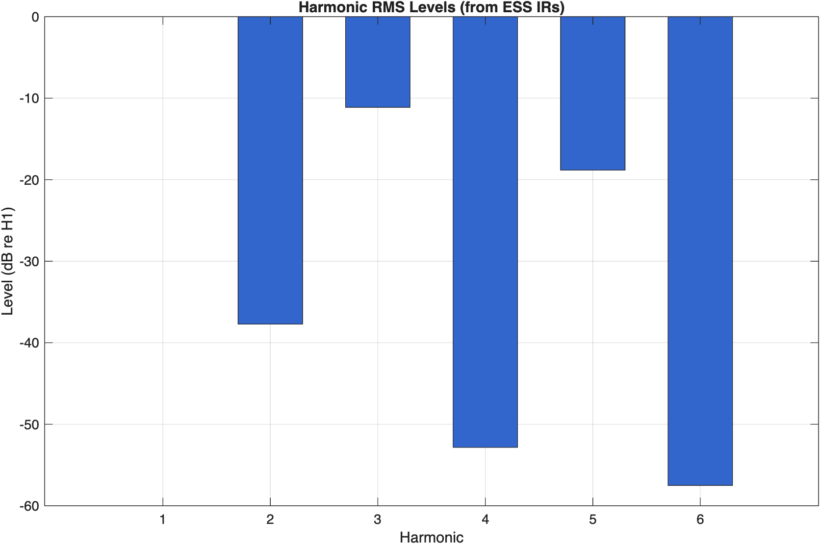
Fig 5 details that the odd harmonics are significantly stronger than the even harmonics, which is resemblant of the behavior of diode based clipping or tanh functions. This means that the Chebyshev model should behave the way that the tanh function is.
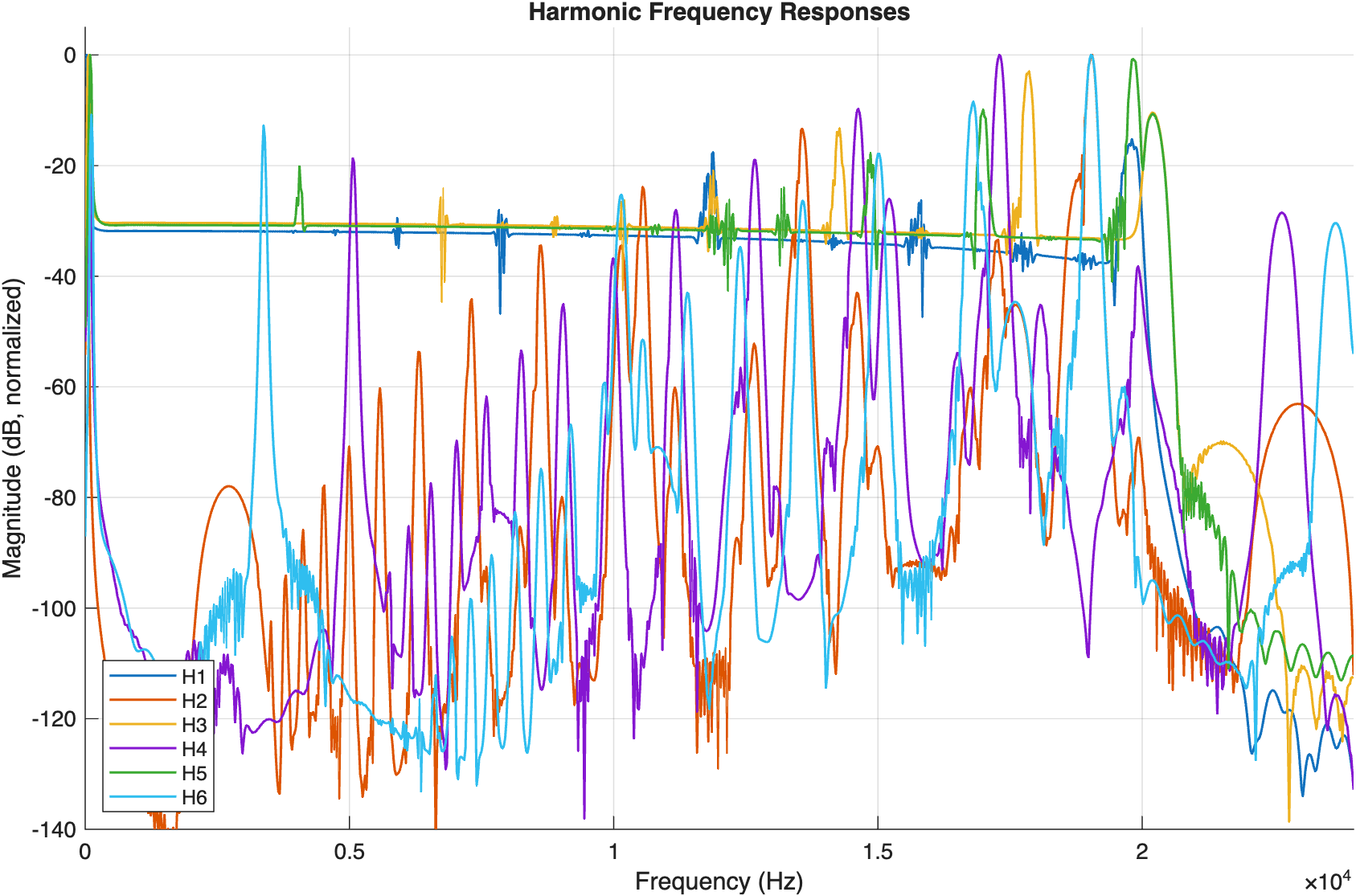
Fig 6: Harmonic Frequency Responses
ESS Discussion
The Chebyshev model was created using an exponential sine sweep, which was used to separate the individual harmonics of the nonlinear system after deconvolution. After the sweep went through the tanh clipper, the output was convolved with a time reversed inverse sine sweep which created these individual harmonics in Matlab. Each harmonic order has a time delay in the deconvolved response which allows for isolation of each harmonic through windowing. The impulse responses are used as filters in a Hammerstein polynomial series where each harmonic order corresponds with the order of the Chebyshev polynomial from the input. This allows the model to reconstruct the nonlinear tanh system by summing all of the filtered polynomials and unlike a Volterra series does not require memory or a summing mixer.
Reflection
In this pre-fx plugin, the “Cheby” switch replaces the tanh clipper with a Chebyshev model that is taken from the file cheby_hk.mat. As seen in fig. 5, the measurements support the assumption that the Chebyshev switch models the behavior of the tanh clipper. As a result, the model can reasonably be used to model the behavior of static nonlinearities in this format.
In fig. 4, the harmonic impulse responses show that the odd harmonics create defined impulse responses, while the even harmonics look noisy. This is not a flaw of the deconvolution process, rather is what is expected from an odd harmonic nonlinearity. Theoretically, the even order harmonics should be zero so the plots reveal noise in the deconvolution process. However, this is insignificant due to the fact that the odd harmonic impulses go significantly over the noise floor. This supports that the Chebyshev model is a strong choice to represent static nonlinearities such as a tanh style distortion at fixed settings. It provides a good approximation of distortion while the even harmonics reveal the noise floor. Additionally, in this plugin, the Chebyshev path does not include the ADAA so it cannot reduce its high frequency harmonic content that will alias.